MCMC diagnostics practice

STA360 at Duke University

Exercises

Exercise 1

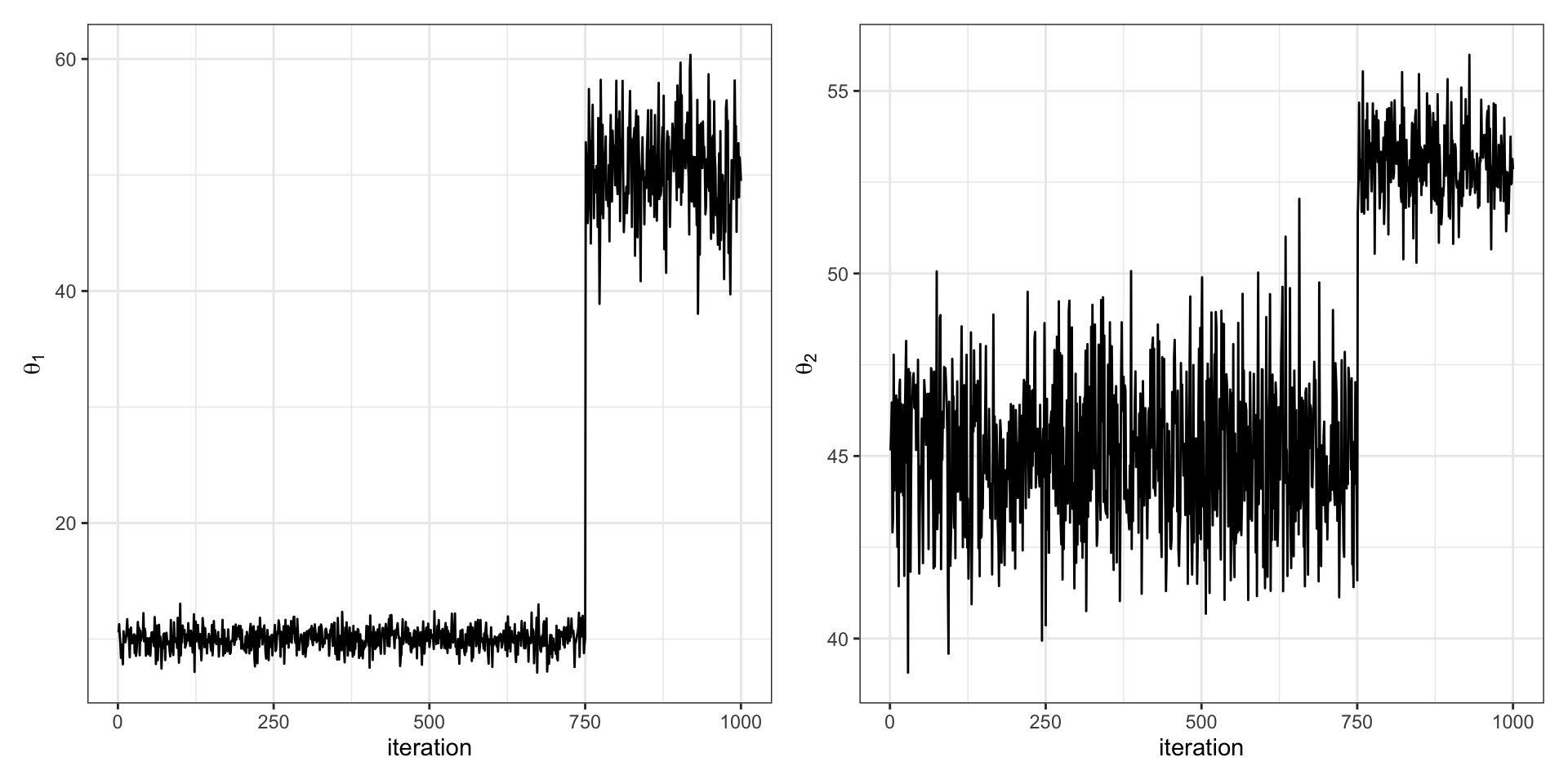
Let \(p(\theta_1, \theta_2 | \mathbf{y})\) be our target distribution, i.e. the distribution we are interested in sampling.

We construct a Gibbs sampler and look at the trace plots of \(\theta_1\) and \(\theta_2\), produced below. Chat with your neighbor, describe what you observe. Has the chain reached stationarity for each parameter? How well is the sampler mixing? Do you think the parameters are correlated or uncorrelated? Why or why not?

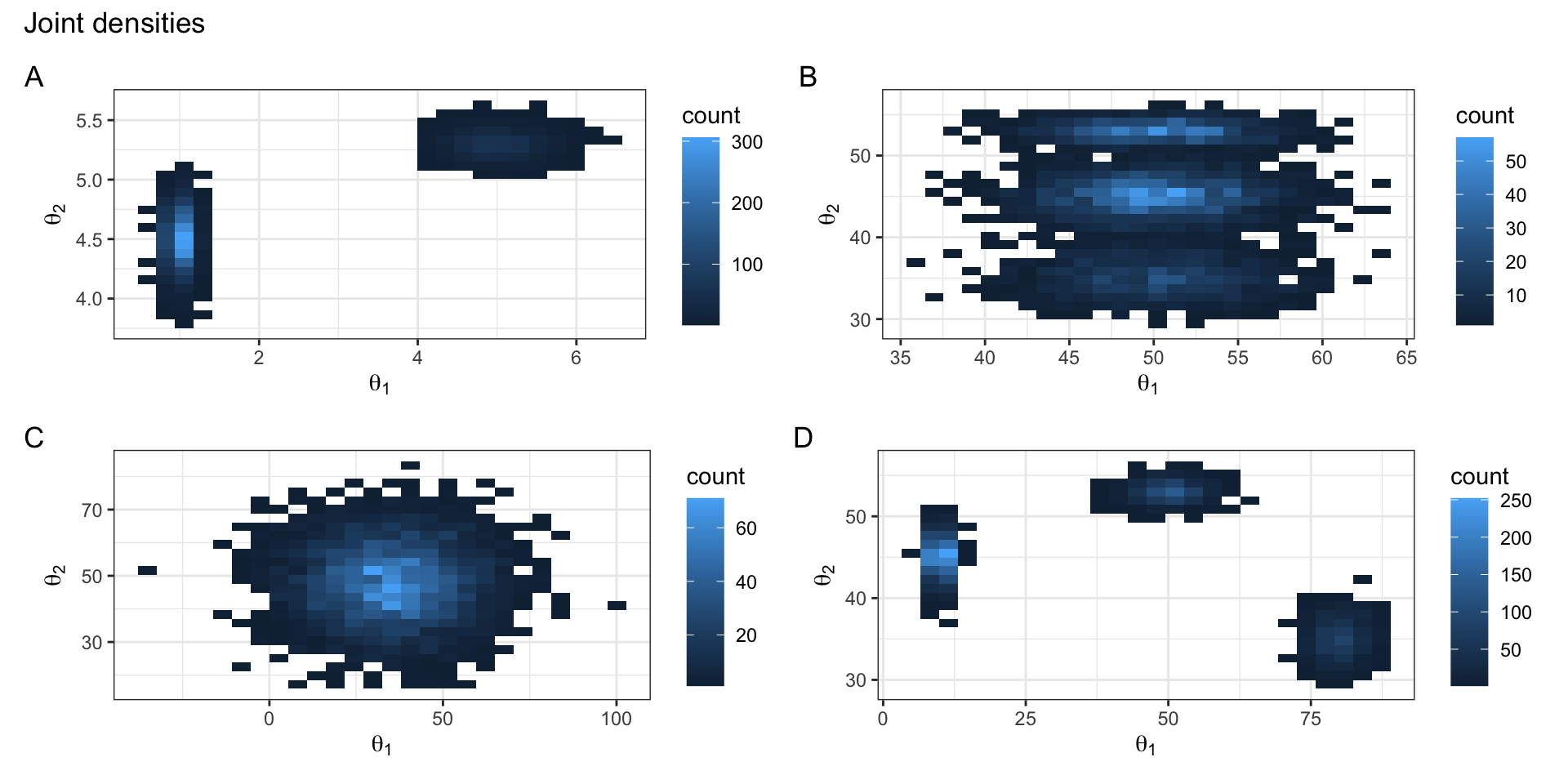
Exercise 2

Based on the first 1000 iterations of your Gibbs sampler shown on the previous slide, which of the following joint densities is the most plausible for \(\theta_1, \theta_2 | \mathbf{y}\)? Why? Hint: it may help to think about where your sampler starts and imagine a particle moving through space according to conditional updates.

Solutions

Solution 1

• The chain has not reached stationarity for either parameter. Different parts of the chain do not look the same.

• Sampler appears to be mixing poorly (at least when run for only 1000 iterations) since we jump from one mode to another only once.

• The parameters look correlated since jumps happen at the same (or nearly the same) iteration.

Solution 2

We start around (10, 45) and up sampling around (50, 53). This rules out (A) and perhaps also (B). Notice the axes.

Plot (C) looks like uncorrelated parameters.

The only plot with islands of high posterior density at these regions is plot (D), which shows an additional mode that we haven’t sampled at all.