rcnorm<-function(n, mean=0, sd=1, a=-Inf, b=Inf){
  u = runif(n, pnorm((a - mean) / sd), pnorm((b - mean) / sd))
  mean + (sd * qnorm(u))
}Homework 8
Due Friday November 22 at 5:00pm
Exercise 1
6.3 from Hoff. You can simulate from a constrained normal distribution with mean mean and standard deviation sd, constrained to lie in the interval \((a,b)\) using the following function:
Note that you can use this function to simulate a vector of constrained normal random variables, each with a potentially different mean, standard deviation, and constraints.
To load the data for this exercise, run the code below
divorce = readr::read_csv("https://sta360-fa24.github.io/data/divorce.csv")Exercise 2
Weighted regression: Suppose \(y_i \sim N(\beta x_i, \sigma^2 / w_i)\) independently for \(i = 1,\ldots n\), where \(x_1, \ldots, x_n\) and \(w_1, \ldots w_n\) are known scalars, and \(\beta\) and \(\sigma^2\) are unknown.
Find the formula for the OLS estimator \(\hat{\beta}_{OLS}\) and compute its variance \(V[\hat{\beta}_{OLS} | \beta, \sigma^2]\).
Write out the sampling density \(p(y_1, \ldots, y_n | \sigma^2, \beta)\) as a function of \(\beta\) (i.e. the likelihood) and find the value of \(\beta\) that maximizes this function (the MLE). Denote this maximizing value as \(\hat{\beta}_{MLE}\). Compute \(V[\hat{\beta}_{MLE} | \beta, \sigma^2]\) and compare it to that of \(\hat{\beta}_{OLS}\).
Under the prior distribution \(\beta \sim N(0, \tau^2)\), find \(E[\beta | y_1, \ldots, y_n, \sigma^2]\). What does this estimator get close to as the prior precision goes to zero (\(\tau^2 \rightarrow \infty\))?
Exercise 3
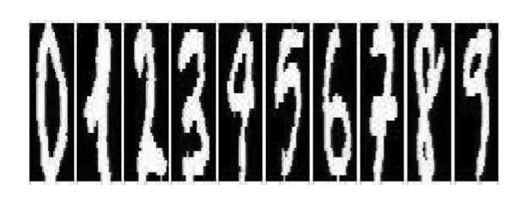
Handwritten digit classification. Data originally sourced from U.S. postal envelopes.
Exercise inspired by Prof. Hua Zhou’s Biostat M280.
In this exercise, you will build a very simple Bayesian image classifier. Load the training and test data sets using the code below.
yTrain = readr::read_csv(
  "https://sta360-fa24.github.io/data/hw-digits-train.csv")

yTest = readr::read_csv(
  "https://sta360-fa24.github.io/data/hw-digits-test.csv"
)
The training data set contains 3822 images like the ones displayed above. Each image is a 32 x 32 bitmap, i.e. 1024 pixels, where each pixel is either black (0) or white (1). The 1024 pixels are divided into 64 blocks of 4 x 4 pixels. Each digit in the data set is represented by a vector of these blocks \(\mathbf{x} = (x_1, \ldots, x_{64})\) where each element is a count of the white pixels in a block (a number between 0 and 16).
The 65th column of the data set (id) is the actual digit label.
How many of each digit are in the training data set? Create a histogram to show the distribution of
block10white pixels for each digit. What do you notice?Assume each digit (i.e. each
id) has its own multinomial data generative model. You can read about the multinomial distribution using?rmultinomin R.
Write down the joint density for images with id “j”, \(\prod_{k = 1}^{n_j} p(\mathbf{x}_k^{(j)} | \boldsymbol{\pi}^{(j)})\). Here \(n_j\) is the number of images of type \(j\) and \(\boldsymbol{\pi}^{(j)} = \{\pi_1^{(j)}, \ldots, \pi_{64}^{(j)} \}\)
How many total unknown parameters are in the complete joint density of all images?
- The Dirichlet distribution is the multivariate generalization of the beta distribution. You can read more about it here. Place a Dirichlet prior on the probability parameters for each of your multinomial models in part b. Let the concentration parameters be all identically 1.
- Sample from the posterior using any method you choose and compute the posterior mean \(\hat{\boldsymbol{\pi}}^{(j)}\) for each \(j\). Hint: you may need to look up how to sample from a Dirichlet distribution in R. You may do this manually or find a package with built-in functions.
- For each image \(\mathbf{x}\) in your testing data set, compute your predicted id according to \(\text{argmax}_{j}~~p(\mathbf{x}| \boldsymbol{\hat{\pi}}^{(j)})p(j)\), where \(p(j)\) is the proportion of digit \(j\) in the training set. Report the number of correct and incorrect classifications in your testing data set.